
Source : Linked in Post
Introduction
In the quantum world, the tiniest mathematical objects can reveal the deepest truths about reality.
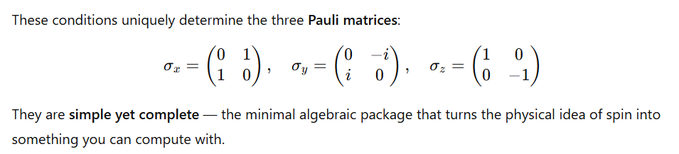
The Pauli matrices — just three little 2×2 grids of numbers — are among the most powerful tools in quantum mechanics.
They form the mathematical DNA of a qubit, describing how it spins, flips, and rotates in its invisible quantum universe.
Understanding these matrices means understanding how a qubit “feels” directions in space — how it responds to measurements, gates, and the fundamental laws that govern quantum information.
⚙️ What Pauli Wanted to Achieve
Physicist Wolfgang Pauli faced a simple but profound question:
How can we describe a two-state quantum system — a spin-½ particle — that changes when we rotate it in space?
Pauli’s goal was to invent a compact algebraic language that captures the behavior of such a system:
a quantum object that can be “up” or “down”, and that transforms nontrivially under rotations.
He needed just three operators to do it — and those became the Pauli matrices.
🧩 Building the Pauli Matrices: From Physical Facts to Mathematical Form
Pauli began from a set of simple, physical requirements. Each one translates naturally into a mathematical property:
| Physical requirement | Mathematical property |
|---|---|
| Give two definite outcomes (up / down) | Operate in a 2D state space → 2×2 matrices |
| Produce real measurement results | Must be Hermitian → real eigenvalues |
| Treat “up” and “down” symmetrically | Must be traceless → eigenvalues ±1 |
| Measuring twice doesn’t change results | Squares to identity matrix |
| Rotations around different axes don’t commute | Must obey SU(2) algebra |
🌐 How They Work: A Visual Intuition
The Pauli matrices correspond to rotations of the Bloch sphere — the geometric model of a qubit’s state.
- σz defines the vertical axis: measuring “up” or “down” (|0⟩ vs |1⟩).
- σx flips the state: moves between |0⟩ and |1⟩.
- σy introduces a phase twist, rotating the qubit in the x–y plane.
Every quantum operation on a single qubit can be seen as a rotation generated by a combination of these matrices.
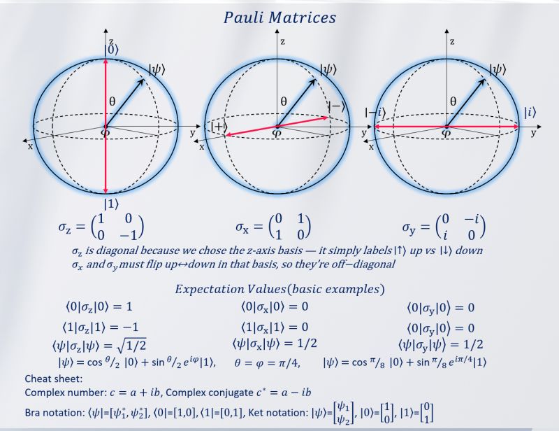
Fig: The three Pauli matrices visualized as rotations on the Bloch sphere. (Source)
🎯 Expectation Values — Where Physics Meets Probability
When you measure a qubit repeatedly along an axis, you get a set of random outcomes — either +1 or −1.
The average of many such measurements is the expectation value, a number between +1 and −1 that tells you how “aligned” the qubit is with that axis.
Example:
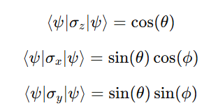
Together, these three numbers form the Bloch vector, giving a full description of the qubit’s state.
In other words:
👉 The Pauli matrices let us turn experimental measurements into a precise mathematical picture.
💡 Why Pauli Matrices Matter for Quantum Computing
Pauli matrices are far more than an abstract algebraic curiosity — they’re the core operating system of every qubit.
Here’s why:
🔁 1. Gates = Rotations
Every quantum gate that acts on a single qubit is a rotation generated by Pauli matrices.
For example:
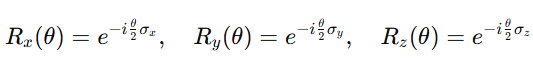
The hardware that drives qubits (microwave pulses, laser beams, etc.) literally implements these rotations in real time.
🧱 2. Building Blocks of Everything
The Pauli matrices form a complete basis for all 2×2 Hermitian operators.
That means you can write any single-qubit Hamiltonian, quantum gate, or noise model as a linear combination of σₓ, σᵧ, and σ_z.
This makes them the universal toolkit for:
- Circuit design
- Simulation
- Quantum control engineering
⚡ 3. Error Description Made Simple
Quantum errors often correspond to one of three basic Pauli flips:
- X error: bit flip
- Y error: bit & phase flip
- Z error: phase flip
This simplicity forms the foundation of Pauli error correction codes, which protect quantum information against noise.
🔍 4. Fast State Tomography & Benchmarking
Measuring expectation values of σₓ, σᵧ, σ_z gives the full Bloch vector.
From that, we can reconstruct the entire state of a qubit — a process called quantum state tomography.
It’s also how we benchmark quantum hardware and validate gate fidelity.
🧮 5. Efficient Simulation & Control
In both theory and experiment, Pauli matrices simplify computation.
They reduce complex quantum dynamics into linear combinations of a few simple terms, making simulation and reasoning faster and more intuitive.
🚀 In Short
The Pauli matrices are the alphabet of the quantum language.
They translate experimental reality — a qubit’s spin, rotation, and phase — into mathematical simplicity.
They tell us:
- How to describe a qubit
- How to rotate it
- How to measure it
- How to correct it
And that’s why these three humble 2×2 matrices appear everywhere — from quantum gates to error correction, from state tomography to quantum machine learning.
🌌 Conclusion
The beauty of the Pauli matrices lies in their minimalism:
three small matrices that capture the essence of quantum reality.
They don’t just describe a qubit —
they define how a qubit feels, interacts, and evolves within its mathematical and physical world.
So next time you see those tiny matrices in a quantum textbook, remember:
they are not just symbols — they are the fingerprints of the quantum universe.
✨ Key Takeaways
| Concept | Meaning |
|---|---|
| Pauli matrices | Fundamental operators describing spin-½ systems |
| Hermitian & traceless | Ensures real, unbiased measurement outcomes |
| Squares to identity | Measuring twice gives the same result |
| SU(2) algebra | Encodes 3D rotational symmetry of qubits |
| Application | Quantum gates, tomography, error correction, and simulation |
🧠 Further Reading
- IBM Quantum Learning: The Bloch Sphere and Pauli Matrices
- Nielsen & Chuang, Quantum Computation and Quantum Information
- Qiskit Textbook: Single-Qubit Gates and the Pauli Basis
Author: Dr. Thyagaraju G. S.
Source: tocxten.com
Exploring the intersection of Quantum Computing, AI, and Conscious Systems.