1. Introduction
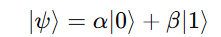
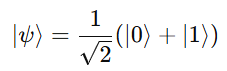
At the heart of quantum computing lies a fundamental concept that defies classical logic — superposition. Unlike a classical bit that can be in only one of two definite states, 0 or 1, a quantum bit (qubit) can exist in a combination, or superposition, of both states simultaneously. This principle enables quantum computers to process a vast number of possibilities at once, leading to unprecedented computational power.
Mathematically, a qubit in superposition is represented as:

2. Representation of Quantum States
Quantum states are expressed using Dirac notation:
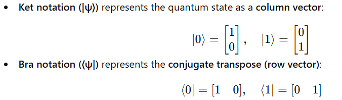
Inner Product
The inner product ⟨ϕ|ψ⟩ gives a scalar indicating the overlap between two quantum states.
Outer Product
The outer product |ψ⟩⟨ϕ| yields a matrix, which is used to construct quantum operators such as projectors and density matrices.
3. Types of Superposition States
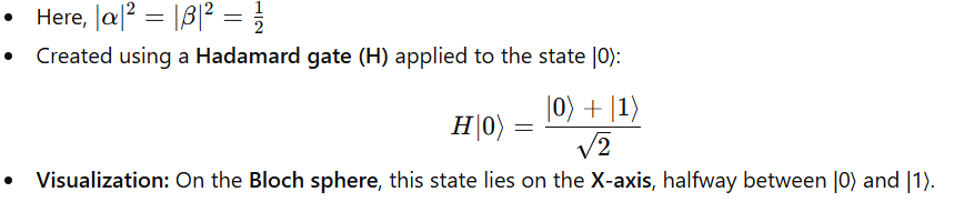
a) Equal Superposition
A qubit has equal probability of being measured as 0 or 1.
b) Biased Towards |0⟩
A state with a higher probability of collapsing to |0⟩:
Example : ∣ψ⟩=0.9∣0⟩+0.435∣1⟩
Here, ∣α∣^2 = 0.81, ∣β^∣2 = 0.19
The qubit is more likely to yield 0 upon measurement.
c) Biased Towards |1⟩
A state with a higher probability of collapsing to |1⟩:
Example : ∣ψ⟩=0.435∣0⟩+0.9∣1⟩
Here, ∣α∣^2 = 0.19, ∣β∣^ 2=0.81
This bias can be generated using a rotation gate, such as Ry(θ), that tilts the qubit closer to |1⟩ on the Bloch sphere.
d) Closer to |0⟩
Intermediate state leaning toward |0⟩, e.g., ∣ψ⟩=0.95∣0⟩+0.312∣1⟩
Measurement is very likely to result in 0.
e) Very Close to |1⟩
∣ψ⟩=0.1∣0⟩+0.995∣1⟩
Measurement is almost certain to give 1.
4. Visualization on the Bloch Sphere
The Bloch Sphere is a 3D geometrical representation of a single qubit’s state.
Each point on the sphere corresponds to a possible qubit state, described as:
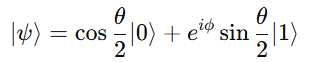
- θ (theta): Polar angle representing the probability distribution.
- φ (phi): Phase angle responsible for interference effects.
- |0⟩ → North Pole (θ = 0)
- |1⟩ → South Pole (θ = π)
- Superpositions lie on the surface between the poles.
The Hadamard gate rotates |0⟩ to the equatorial plane, creating equal superposition — a crucial step for quantum parallelism.
Qiskit Program: Bloch Sphere Visualization of θ and φ
# Visualizing Qubit States on the Bloch Sphere (θ & φ)
This notebook demonstrates:
- The Bloch-sphere representation of a single qubit.
- How θ (polar) and φ (azimuthal/phase) determine the qubit state.
- |0⟩ at the North pole (θ=0) and |1⟩ at the South pole (θ=π).
- Superpositions on the equator and the effect of φ (phase).
- How the Hadamard gate moves |0⟩ to the equator (equal superposition).
- A measurement histogram for H|0⟩ using AerSimulator.

**Instructions:** Run cells in order in a Jupyter Notebook. Requires `qiskit` and `qiskit-aer`.
# Cell 2: Imports and notebook plotting setup

%matplotlib inline

import numpy as np
import matplotlib.pyplot as plt
from IPython.display import display, HTML

from qiskit import QuantumCircuit
from qiskit.quantum_info import Statevector
from qiskit.visualization import plot_bloch_vector, plot_histogram
from qiskit_aer import AerSimulator

# Clear existing matplotlib figures (avoid leftover empty plots)
plt.close('all')
Explanation:
Load required libraries, configure inline plotting for Jupyter, and close stray figures to avoid empty boxes.
# Cell 3: Helper functions to compute and plot Bloch vectors

def bloch_coords_from_statevector(state: Statevector):
    """
    Convert a single-qubit Statevector to Bloch coordinates [x, y, z].
    state.data is a length-2 complex array: [a, b] representing a|0> + b|1>.
    """
    a = state.data[0]
    b = state.data[1]
    x = 2 * np.real(a * np.conj(b))
    y = 2 * np.imag(a * np.conj(b))
    z = np.abs(a)**2 - np.abs(b)**2
    return [x, y, z]

def plot_state_on_bloch(qc: QuantumCircuit, title: str = None):
    """
    Given a single-qubit circuit (no measurements), compute its Statevector,
    convert to Bloch coordinates, and plot using plot_bloch_vector.
    Returns (fig, state).
    """
    state = Statevector.from_instruction(qc)
    vec = bloch_coords_from_statevector(state)
    fig = plot_bloch_vector(vec)   # returns a matplotlib.figure.Figure
    if title:
        fig.suptitle(title, fontsize=12)
    display(fig)
    return fig, state

def show_circuit(qc: QuantumCircuit, title: str = None):
    """Display the circuit diagram (matplotlib) with an optional title."""
    if title:
        display(HTML(f"<b>{title}</b>"))
    display(qc.draw('mpl'))
Explanation:
bloch_coords_from_statevector: converts state amplitudes to Bloch (x,y,z).plot_state_on_bloch: uses the above andplot_bloch_vectorto produce a robust figure.show_circuit: displays the circuit diagram for clarity.
Case A — The ground state |0⟩ (North Pole, θ = 0)
No gates applied; the qubit is in |0⟩, which corresponds to the North Pole on the Bloch sphere.
# Cell 4: |0> state

qc_0 = QuantumCircuit(1)   # no gates -> |0>
fig0, state0 = plot_state_on_bloch(qc_0, title="|0⟩ → North Pole (θ = 0)")
show_circuit(qc_0, title="Circuit for |0⟩ (no gates)")
display(state0.draw('latex'))   # show the ket in LaTeX form
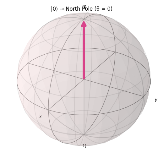
Explanation:
This shows the Bloch vector pointing up; the statevector should be [1, 0].
Case B — The excited state |1⟩ (South Pole, θ = π)
Apply an X gate to flip |0⟩ → |1⟩. This state maps to the South Pole on the Bloch sphere.
# Cell 5: |1> state

qc_1 = QuantumCircuit(1)
qc_1.x(0)   # X gate flips to |1>
fig1, state1 = plot_state_on_bloch(qc_1, title="|1⟩ → South Pole (θ = π)")
show_circuit(qc_1, title="Circuit for |1⟩ (X gate)")
display(state1.draw('latex'))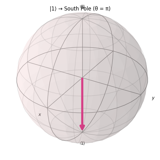
Explanation:
X rotates the state from north to south; statevector should be [0,1].
Case C — Equal superposition along the X-axis (θ = π/2, φ = 0)
Prepare the state with Ry(π/2) or directly using the Hadamard gate. This puts the Bloch vector on the equator pointing along +X.
# Cell 6: Superposition on X-axis using Ry(π/2)

qc_sup_x = QuantumCircuit(1)
qc_sup_x.ry(np.pi/2, 0)   # rotate from |0> down to equator (theta=pi/2)
fig_sup_x, state_sup_x = plot_state_on_bloch(qc_sup_x, title="Superposition (θ = π/2, φ = 0) → X-axis")
show_circuit(qc_sup_x, title="Circuit: Ry(π/2) (equator, φ=0)")
display(state_sup_x.draw('latex'))
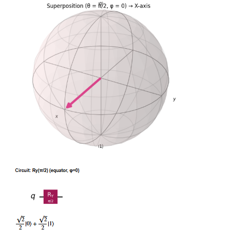
Explanation:Ry(π/2) moves the vector from the North Pole to the equator; probabilities for |0⟩ and |1⟩ are both 0.5.
Case D — Superposition on the equator with phase (θ = π/2, φ = π/2)
Apply Ry(π/2) then Rz(π/2). The Rz adds relative phase φ, rotating the equatorial point around the Z axis (e.g., moves from X-axis towards Y-axis).
# Cell 7: Superposition with phase

qc_sup_y = QuantumCircuit(1)
qc_sup_y.ry(np.pi/2, 0)
qc_sup_y.rz(np.pi/2, 0)    # adds phase φ = π/2
fig_sup_y, state_sup_y = plot_state_on_bloch(qc_sup_y, title="Superposition (θ = π/2, φ = π/2) → Y-axis")
show_circuit(qc_sup_y, title="Circuit: Ry(π/2) then Rz(π/2)")
display(state_sup_y.draw('latex'))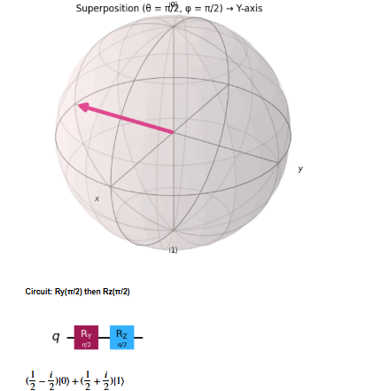
Explanation:
This demonstrates that φ changes the azimuthal angle — interference behavior depends on phase, even though probabilities remain 50/50.
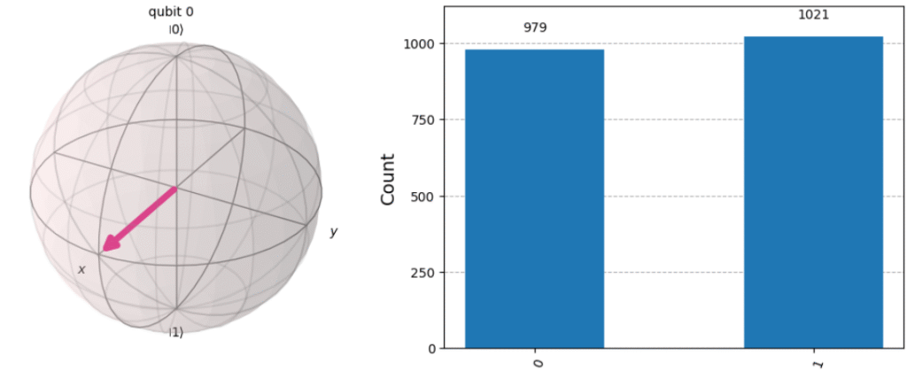
Case E — Hadamard on |0⟩ → equal superposition
Apply H to |0⟩. H maps |0⟩ to (|0⟩ + |1⟩)/√2 which is on the equator (θ = π/2) along the X-axis.
# Cell 8: Hadamard effect

qc_h = QuantumCircuit(1)
qc_h.h(0)
fig_h, state_h = plot_state_on_bloch(qc_h, title="Hadamard on |0⟩ → Equal superposition on equator")
show_circuit(qc_h, title="Circuit: H on |0⟩")
display(state_h.draw('latex'))
Explanation:
Hadamard is commonly used to create quantum parallelism by placing qubits in equal superposition.
Measurement demonstration (histogram)
Create the same H|0⟩ state but in a circuit with a classical bit and measure it many times using AerSimulator.
This shows the probabilistic collapse: counts should be ≈ 50% |0⟩ and 50% |1⟩.
# Cell 9: Measurement histogram using a separate circuit with a classical bit

qc_measure = QuantumCircuit(1, 1)
qc_measure.h(0)
qc_measure.measure(0, 0)

show_circuit(qc_measure, title="Measurement circuit (H then measure)")

# Run simulation
sim = AerSimulator()
job = sim.run(qc_measure, shots=2000)
result = job.result()
counts = result.get_counts()

fig_hist = plot_histogram(counts)
fig_hist.suptitle("Measurement outcomes (shots=2000) for H|0⟩", fontsize=12)
display(fig_hist)

print("Counts:", counts)
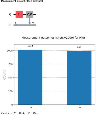
Explanation:Statevector can’t be used on circuits with measurements. We use a separate circuit with classical bits for the measurement step and AerSimulator to collect frequencies.
Parameterized state builder
Helper to construct a state for arbitrary θ and φ:
|ψ⟩ = cos(θ/2)|0⟩ + e^{iφ} sin(θ/2)|1⟩
We implement this by Ry(θ) followed by Rz(φ).
Try different θ and φ values interactively.
# Cell 10: Parameterized circuit from theta and phi
def circuit_from_theta_phi(theta, phi):
    qc = QuantumCircuit(1)
    qc.ry(theta, 0)
    qc.rz(phi, 0)
    return qc

# Example: custom θ and φ
theta_example = np.pi/3   # 60 degrees
phi_example = np.pi/4     # 45 degrees
qc_custom = circuit_from_theta_phi(theta_example, phi_example)
fig_custom, state_custom = plot_state_on_bloch(qc_custom, title=f"Custom: θ={theta_example:.2f}, φ={phi_example:.2f}")
show_circuit(qc_custom, title="Circuit: Ry(theta) then Rz(phi)")
display(state_custom.draw('latex'))

Explanation:
Use this to explore arbitrary positions on the Bloch sphere. You can vary θ in [0, π] and φ in [0, 2π].
5. Real-Time Example Using Qiskit
Here’s how to create and visualize superposition in Qiskit (Jupyter Notebook ready):
%matplotlib inline
from qiskit import QuantumCircuit
from qiskit.quantum_info import Statevector
from qiskit_aer import AerSimulator
from qiskit.visualization import plot_bloch_multivector, plot_histogram
import matplotlib.pyplot as plt
from IPython.display import HTML
import io
from base64 import b64encode

# --- prepare state (no measurements) and get Bloch fig ---
qc_state = QuantumCircuit(1)
qc_state.h(0)
state = Statevector.from_instruction(qc_state)
fig1 = plot_bloch_multivector(state)   # returns a matplotlib.figure.Figure

buf1 = io.BytesIO()
fig1.savefig(buf1, format='png', bbox_inches='tight')
buf1.seek(0)
img1_b64 = b64encode(buf1.read()).decode('ascii')
plt.close(fig1)

# --- prepare measured circuit and histogram fig ---
qc_measure = QuantumCircuit(1, 1)
qc_measure.h(0)
qc_measure.measure(0, 0)

sim = AerSimulator()
result = sim.run(qc_measure, shots=2000).result()
counts = result.get_counts()

fig2 = plot_histogram(counts)  # this also returns a Figure
buf2 = io.BytesIO()
fig2.savefig(buf2, format='png', bbox_inches='tight')
buf2.seek(0)
img2_b64 = b64encode(buf2.read()).decode('ascii')
plt.close(fig2)

# --- render both images side-by-side in notebook output ---
html = f"""
<div style="display:flex; align-items:flex-start; gap:20px;">
  <div><img src="data:image/png;base64,{img1_b64}" /></div>
  <div><img src="data:image/png;base64,{img2_b64}" /></div>
</div>
"""
display(HTML(html))
6. Applications of Superposition
a) Quantum Parallelism
Superposition enables a quantum computer to evaluate multiple inputs simultaneously — a core principle behind algorithms like:
- Shor’s algorithm for factorization,
- Grover’s search algorithm for database searching.
b) Quantum Communication
In Quantum Key Distribution (QKD) (e.g., BB84 protocol), superposed states are used to encode cryptographic keys that are impossible to intercept without detection.
c) Quantum Sensors
Superposition-based sensors can detect minuscule changes in physical quantities such as magnetic fields, gravity, or time with ultra-high sensitivity (used in atomic clocks and MRI).
d) Quantum Neural Networks
Superposition allows quantum neurons to represent multiple states at once, enhancing pattern recognition and decision-making capabilities.
e) Real-Time Control Systems
In emerging Quantum AI systems, superposition is exploited to model uncertainty and probabilistic reasoning in smart traffic lights, autonomous vehicles, and financial modeling.
7. Conclusion
The superposition of qubits forms the foundation of all quantum computation. It transforms binary thinking into a continuous spectrum of probabilities, enabling algorithms to explore multiple outcomes simultaneously. From secure communication to intelligent control systems and advanced computation, superposition is not merely a quantum concept — it is the bridge between classical limits and quantum possibilities.