1. Introduction
In quantum computing, quantum gates are the fundamental building blocks used to manipulate quantum bits or qubits. Just as classical logic gates (like AND, OR, NOT) operate on bits, quantum gates operate on qubits to change their state. However, unlike classical gates, quantum gates are reversible and operate on superpositions of states, enabling powerful computations that classical computers cannot efficiently perform.
A single-qubit gate acts on one qubit at a time. These gates can:
- Rotate the qubit’s state on the Bloch Sphere.
- Flip the qubit between its basis states |0⟩ and |1⟩.
- Change the phase of the qubit’s state.
- Create or destroy superposition states.
Each single-qubit gate can be represented by a 2×2 unitary matrix. A unitary matrix U satisfies the condition: U†U=I
where U†U^\daggerU† is the conjugate transpose of UUU, and III is the identity matrix. This ensures that quantum operations preserve probability (the total probability always remains 1).
Why Single-Qubit Gates Are Important
Single-qubit gates form the foundation for all quantum operations. By combining them with multi-qubit gates such as the CNOT gate, we can build any complex quantum algorithm. Thus, mastering single-qubit gates is the first step toward understanding quantum computation and quantum circuit design.
In this chapter, we will explore the mathematical representation, purpose, and Qiskit implementations of the key single-qubit gates:
- Pauli-X Gate
- Pauli-Y Gate
- Pauli-Z Gate
- Hadamard Gate
- Phase Shift Gate
We will also examine their effects on basic and superposed states, visualize results on the Bloch Sphere, and finally perform a comparative analysis to understand their relationships
2. Mathematical Representation of Qubit Gates
To understand how single-qubit gates work, it’s important to first understand the mathematical representation of qubits and how gates act upon them.
2.1 Qubit Representation
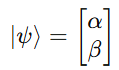
A qubit is the quantum equivalent of a classical bit. While a classical bit can only exist in one of two states (0 or 1), a qubit can exist in a superposition of both:
∣ψ⟩=α∣0⟩+β∣1⟩
where
- α and β are complex probability amplitudes,
- ∣α∣^2 and ∣β∣^2 represent the probabilities of measuring the qubit in states |0⟩ and |1⟩ respectively, and they must satisfy the normalization condition: ∣α∣^2 + ∣β∣^2 = 1
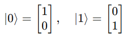
2.2 Matrix Form of Basis States
We can express the basis states as column vectors:
Thus, any qubit ∣ψ⟩ can be written as:
2.3 Quantum Gate as a Matrix
A quantum gate acts on qubits via matrix multiplication.
If U is the matrix representing a quantum gate, then:
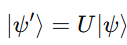
Here, ∣ψ′⟩|\psi’\rangle∣ψ′⟩ is the new quantum state after applying the gate.
Since UUU must be unitary, it guarantees reversibility and probability conservation.
2.4 Example
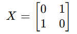
Let’s take a simple example — the Pauli-X gate, also called the quantum NOT gate.
It is represented as:
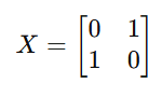
When it acts on ∣0⟩|0\rangle∣0⟩:
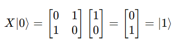
and vice versa:
X∣1⟩=∣0⟩
This shows that the Pauli-X gate flips the qubit, similar to a classical NOT operation.
2.5 Bloch Sphere Interpretation
Every single-qubit state can also be represented as a point on the Bloch Sphere, where:
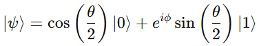
Here,
- θ and ϕ are spherical coordinates that define the qubit’s position on the sphere.
- Quantum gates correspond to rotations on this sphere.
Thus, each single-qubit gate can be interpreted as a rotation operator acting on the Bloch Sphere.
2.6 Unitarity, Hermitian Property, and Reversibility
In quantum mechanics, every operation that evolves a quantum state must preserve total probability. This requirement is mathematically guaranteed if the operator (gate) is unitary.
Unitarity
A matrix U is unitary if:
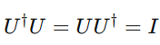
where
- U† is the conjugate transpose (Hermitian adjoint) of U,
- III is the identity matrix.
This ensures that the transformation does not change the overall length (magnitude) of the quantum state vector.
Hence, the probabilities remain normalized — total probability = 1.
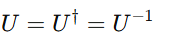
Because a unitary matrix has an inverse equal to its conjugate transpose
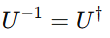
it follows that every quantum operation is reversible.
This is a major distinction from classical logic gates (e.g., AND, OR), which are generally irreversible because they lose information.
Hermitian Property
A matrix H is Hermitian if:

Hermitian matrices play a special role in quantum mechanics:
- They represent observable quantities (like energy, spin, momentum).
- When a gate’s matrix is both unitary and Hermitian, it implies:
meaning that applying the same gate twice restores the original state.
For example:
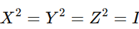
This shows that applying Pauli gates twice is equivalent to doing nothing — they are self-inverse and therefore Hermitian as well as unitary.
3. List of All Single-Qubit Gates and Their Purpose
Single-qubit gates form the foundation of quantum computation. They manipulate a single qubit’s state by rotating or phase-shifting it on the Bloch Sphere. Each gate corresponds to a specific unitary matrix that defines how the qubit state transforms.
Below is an overview of the most important single-qubit gates used in quantum computing:
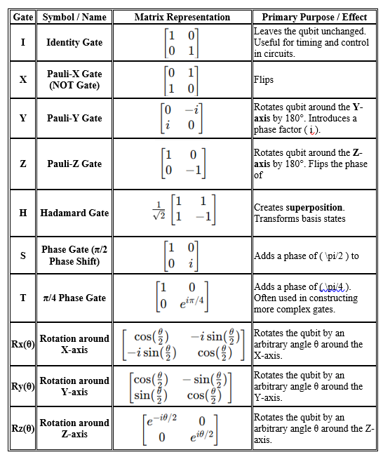
3.1 Observations
- All these gates are unitary, ensuring reversibility.
- Pauli-X, Y, Z gates represent 180° rotations around the respective axes of the Bloch sphere.
- Hadamard and Phase gates are essential for creating superpositions and phase shifts, key ingredients in quantum interference.
- Rotation gates generalize Pauli gates by allowing continuous transformations.
3.2 Classification
Single-qubit gates can be broadly classified into:
- Pauli Gates (X, Y, Z) — Basic rotation operators
- Superposition Gate (H) — Creates quantum superposition
- Phase Gates (S, T, Rz) — Control and modify phase relationships
These gates, when combined with at least one two-qubit entangling gate (like CNOT), are universal — meaning they can build any possible quantum operation.
4. Pauli-X Gate
4.1 Definition
The Pauli-X gate, also known as the Quantum NOT Gate, performs a bit-flip operation on a qubit.
It flips the state |0⟩ to |1⟩ and |1⟩ to |0⟩ — analogous to the classical NOT gate in digital logic.
Mathematically, the Pauli-X gate is one of the Pauli matrices and represents a rotation of π radians (180°) about the X-axis of the Bloch sphere.
4.2 Matrix Representation and Properties
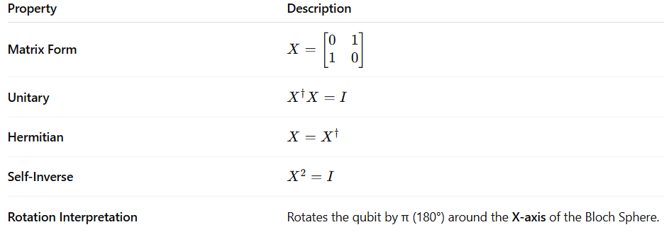
Thus, applying the X gate twice brings the qubit back to its original state.
X(X∣ψ⟩)=∣ψ⟩
4.3 Effect on Basis States
Let’s apply the X gate on the two computational basis states:
X∣0⟩=∣1⟩, X∣1⟩=∣0⟩
That is, it flips the basis states — a quantum version of NOT operation.
4.4 Effect on Superposition States
For a general qubit: ∣ψ⟩=α∣0⟩+β∣1⟩
the Pauli-X gate gives:
X∣ψ⟩=αX∣0⟩+βX∣1⟩=α∣1⟩+β∣0⟩
Hence, it swaps the amplitudes of |0⟩ and |1⟩.
If we apply it to a Hadamard-created superposition:
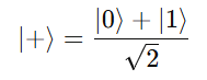
then
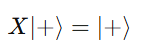
So, |+⟩ is an eigenstate of X with eigenvalue +1.
4.5 Qiskit Example: Pauli-X Gate
Below is a complete example in Qiskit that shows the effect of the Pauli-X gate on |0⟩ and on a superposed qubit.
# Import necessary modules
from qiskit import QuantumCircuit
from qiskit.visualization import plot_histogram
from qiskit_aer import AerSimulator
from qiskit.visualization import plot_bloch_multivector

# Create a Quantum Circuit with one qubit and one classical bit
qc = QuantumCircuit(1, 1)

# Apply X gate
qc.x(0)

# Measure the qubit
qc.measure(0, 0)

# Display the circuit
qc.draw('mpl')
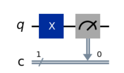
Explanation:
- The circuit starts with the qubit in state |0⟩.
- The X gate flips it to |1⟩.
- Measurement confirms the result is always 1.
Now let’s see the effect on a superposed qubit created using a Hadamard gate:
import matplotlib
import sys
print("matplotlib backend:", matplotlib.get_backend())
print("python executable:", sys.executable)

# If you're in a notebook, this will import display() for later use
from IPython.display import display
# Run this in a notebook cell
%matplotlib inline
# Then (same as before)
from qiskit import QuantumCircuit, transpile
from qiskit_aer import AerSimulator
from qiskit.visualization import plot_bloch_multivector
import matplotlib.pyplot as plt
qc2 = QuantumCircuit(1)
qc2.h(0); qc2.x(0)
qc2.save_statevector()
sim = AerSimulator()
tqc = transpile(qc2, sim)
result = sim.run(tqc).result()
statevector = result.get_statevector()
fig = plot_bloch_multivector(statevector) # returns a matplotlib.figure.Figure
display(fig) # explicit display in notebooks
# plt.show() # not necessary when using display(fig)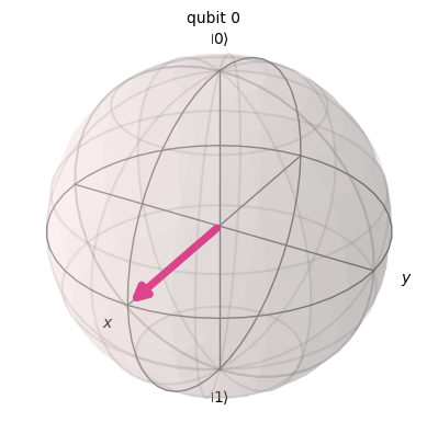
Explanation:
- The Hadamard gate creates a superposition (|0⟩ + |1⟩)/√2.
- The X gate swaps amplitudes, but since both are equal, the state remains unchanged on the Bloch sphere along the X-axis.
5. Pauli-Y Gate
5.1 Definition
The Pauli-Y gate is one of the three fundamental Pauli matrices used in quantum computing.
It represents a π (180°) rotation about the Y-axis on the Bloch sphere.
While the Pauli-X gate flips the qubit between |0⟩ and |1⟩ (bit flip), the Pauli-Y gate performs a bit flip combined with a phase shift.
Mathematically, it introduces a complex phase factor (i) that distinguishes it from the X gate.
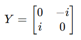
5.2 Matrix Representation
The Pauli-Y gate is represented by the following 2×2 unitary and Hermitian ma
| Property | Description |
|---|---|
| Unitary | ( Y^† Y = I ) |
| Hermitian | ( Y = Y^† ) |
| Self-Inverse | ( Y^2 = I ) |
| Rotation | Rotation of π around Y-axis |
5.3 Effect on Basis States
Let’s apply Y to the computational basis states:
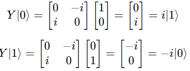
Hence,
- |0⟩ → i|1⟩
- |1⟩ → –i|0⟩
So it performs a bit flip with a phase factor of ±i.
5.4 Effect on Superposition States
For a general qubit: ∣ψ⟩=α∣0⟩+β∣1⟩
The Pauli-Y operation gives: Y∣ψ⟩=α(i∣1⟩)+β(−i∣0⟩)=−i(β∣0⟩−α∣1⟩)
This shows that the Y gate not only flips the amplitudes but also introduces a phase rotation of ±i, representing a 180° rotation about the Y-axis on the Bloch sphere.
5.5 Qiskit Example: Pauli-Y Gate
Below is a complete example you can run directly in Jupyter Notebook (with inline visualization):
# Ensure inline plotting for Jupyter Notebook
%matplotlib inline

# Import required libraries
from qiskit import QuantumCircuit, transpile
from qiskit_aer import AerSimulator
from qiskit.visualization import plot_bloch_multivector, plot_histogram
import matplotlib.pyplot as plt

# Create Quantum Circuit
qc = QuantumCircuit(1, 1)

# Apply Y gate to |0>
qc.y(0)

# Display the circuit
qc.draw('mpl')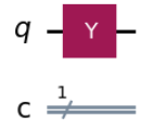
🧠 Explanation:
- The circuit starts with the qubit in state |0⟩.
- Applying the Y gate rotates the qubit 180° about the Y-axis.
- The resulting state is i|1⟩, equivalent to |1⟩ up to a global phase.
5.6 Visualization of Pauli-Y on Superposed State
Now let’s visualize the effect of Y on a superposition created by the Hadamard gate.
# Create a new circuit for visualization
qc2 = QuantumCircuit(1)
qc2.h(0)  # Create superposition (|0> + |1>)/√2
qc2.y(0)  # Apply Pauli-Y gate
qc2.save_statevector()  # Save the quantum state

# Simulate
sim = AerSimulator()
tqc2 = transpile(qc2, sim)
result = sim.run(tqc2).result()

# Get the statevector
statevector = result.get_statevector()

# Plot Bloch vector
fig = plot_bloch_multivector(statevector)
display(fig)  # Ensures inline output in Jupyter
✅ Expected Result:
- The qubit rotates around the Y-axis by 180°, moving the state from +X to –X direction on the Bloch sphere.
- You’ll see the point shift to the opposite side of the sphere along the X-axis.