1. Introduction
In 1925, Werner Heisenberg introduced a revolutionary way to describe quantum systems — known as the Matrix Mechanics formulation of quantum mechanics.
Unlike classical physics, where we describe the motion of a particle using definite paths (trajectories), Heisenberg proposed that the physical world at the atomic scale cannot be described in terms of definite positions and velocities.
Instead, the observable quantities such as position, momentum, and energy should be represented as mathematical matrices, whose elements describe transitions between different energy states of a quantum system.
This approach marked the beginning of modern quantum mechanics, and it was later shown by Schrödinger that his wave mechanics and Heisenberg’s matrix mechanics are mathematically equivalent.
2. Historical Background
Before 1925, physicists were struggling to explain the behavior of atomic spectra — such as the discrete spectral lines of hydrogen.
Bohr’s model could explain only some of these lines but not the detailed structure or intensity patterns.
Heisenberg, while working under Niels Bohr, realized that the theory should only deal with observable quantities like spectral frequencies and intensities, rather than unobservable “electron orbits.”
Thus, he constructed a new mathematical framework — Matrix Mechanics — where the physical quantities are replaced by arrays of numbers (matrices) that encode the probabilities of transitions between quantum states.
3. Fundamental Idea
In classical mechanics: x(t), p(t)
represent position and momentum of a particle as functions of time.
In quantum mechanics (Matrix Formulation): X, P
represent position and momentum operators, which are matrices instead of simple numbers.
Each matrix element corresponds to a possible transition between two quantum states.
Example: Position Matrix
Suppose a particle can exist only in two energy states, ∣1⟩ and ∣2⟩.
Then the position operator X can be represented as:
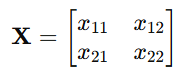
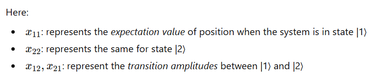
These elements can be complex numbers.
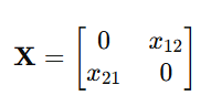
4. Matrix Representation of Observables
Every observable quantity (like position, momentum, energy) in quantum mechanics is represented by a Hermitian matrix (or operator) because physical observables always have real eigenvalues.
Examples:
(a) Position Operator:
(b) Momentum Operator:
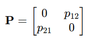
These matrices are related through commutation relations.
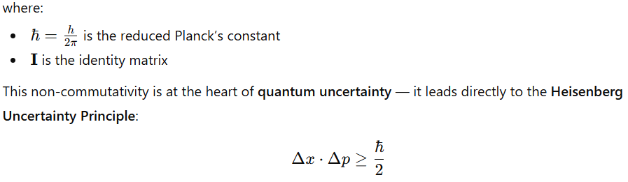
5. The Fundamental Commutation Relation
Heisenberg discovered that position and momentum matrices do not commute:
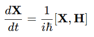
6. Time Evolution in Matrix Mechanics
In Matrix Mechanics, the time dependence of an observable A\mathbf{A}A (like position or momentum) is given by the Heisenberg Equation of Motion:
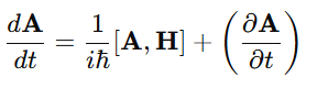
where H is the Hamiltonian matrix (total energy operator). This equation plays a similar role to Newton’s law in classical mechanics.
Example:
For a free particle (no potential energy),
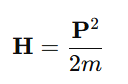
Then the time evolution of position is:
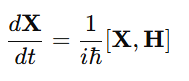
which gives:
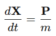
This is analogous to the classical relation v=p/m.
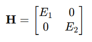
7. Example: Two-Level Quantum System
Consider a system with two energy levels: E1,E2
and the energy operator (Hamiltonian) as:
If X is the position matrix:
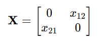
Then:
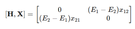
According to Heisenberg’s equation of motion:
Thus, the matrix elements oscillate with a frequency proportional to the energy difference (E2−E1)/ℏ
This perfectly explains spectral line frequencies in atoms — one of the original motivations for Heisenberg’s theory.
8. Relationship with Schrödinger’s Wave Mechanics
In 1926, Erwin Schrödinger developed his wave mechanics, where physical systems are described by wavefunctions.
It was later proved that:
Heisenberg’s Matrix Mechanics and Schrödinger’s Wave Mechanics are mathematically equivalent.
In matrix mechanics, states are represented as column vectors (state vectors), and observables as operators (matrices) that act on them.
This led to the modern Dirac formulation using bra–ket notation:
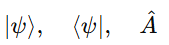
where:

gives the expectation value of observable A.
9. Significance of Heisenberg’s Matrix Formulation
- It introduced the idea that observables are operators, not numerical quantities.
- It naturally led to the Uncertainty Principle.
- It was the first complete formulation of quantum mechanics.
- It laid the foundation for quantum computation, quantum information, and operator algebra in physics.
10. Summary
| Concept | Classical Mechanics | Heisenberg’s Matrix Mechanics |
|---|---|---|
| Variables | Numbers | Matrices (operators) |
| Observables | Definite values | Expectation values |
| Motion law | Newton’s laws | Heisenberg’s equation of motion |
| Commutation | Variables commute | Operators don’t commute |
| Determinism | Deterministic | Probabilistic |
| Example | (x, p) | X,P |
11. Conclusion
Heisenberg’s Matrix Formulation fundamentally changed our understanding of nature.
It showed that, at the quantum level, the world is not deterministic, but governed by probabilities and observable transitions between quantized states.
Matrix mechanics, together with wave mechanics and Dirac’s formulation, forms the complete mathematical framework of quantum mechanics that underpins modern physics, chemistry, and quantum computing.
12. Suggested Reading
- Heisenberg, W. (1925). Quantum-Theoretical Re-Interpretation of Kinematic and Mechanical Relations.
- Dirac, P.A.M. (1930). Principles of Quantum Mechanics.
- Griffiths, D. (2018). Introduction to Quantum Mechanics.
- Feynman, R.P. (1965). The Feynman Lectures on Physics, Vol. III.